Lesson 10 of 16 · 41:41
Sorting algorithms
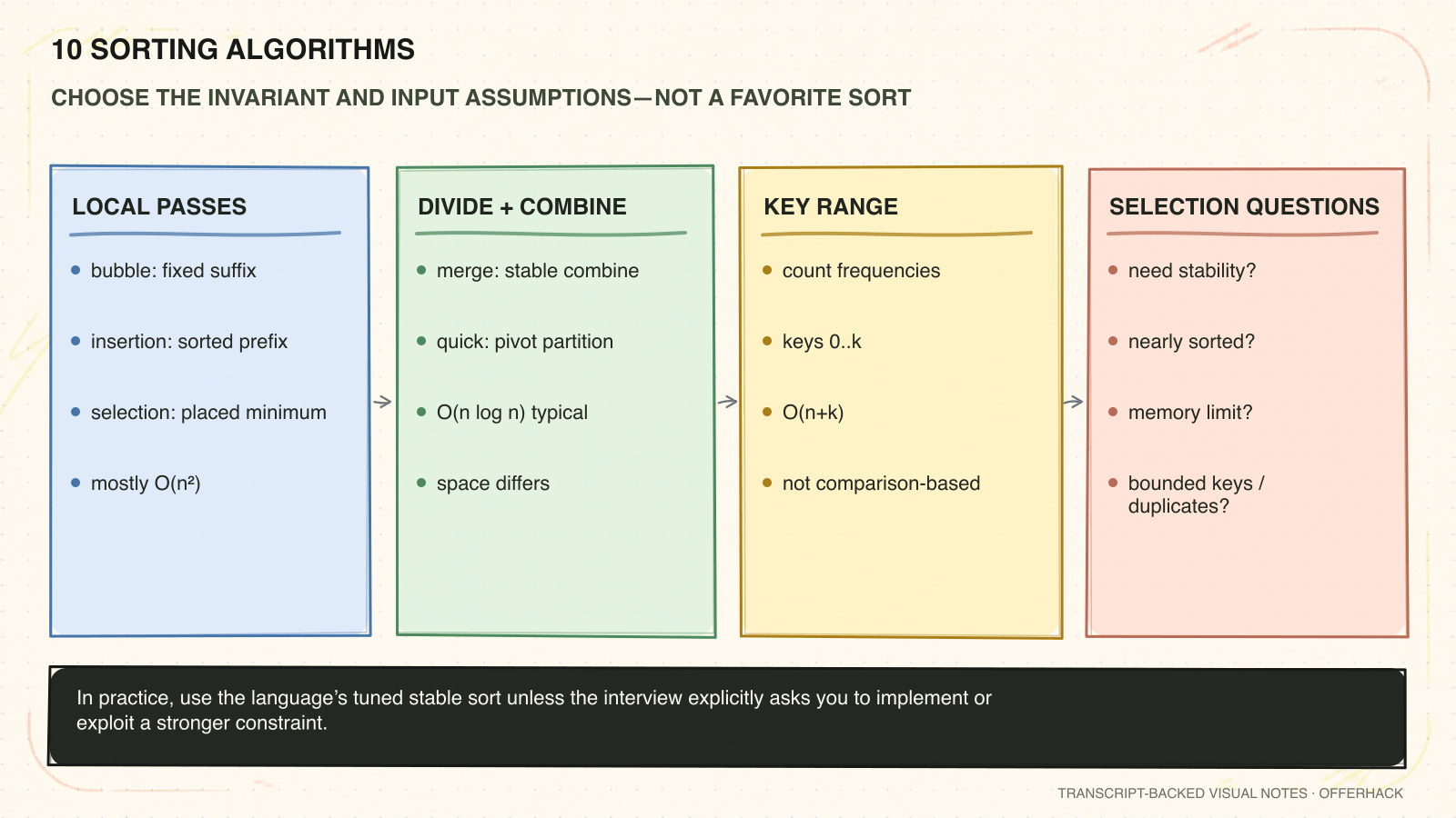
Sorting algorithms reveal several reusable ideas: grow a proven sorted region, merge ordered streams, or partition values around a pivot. In interviews, you rarely need to hand-code every elementary sort, but you do need to recognize how sorting changes a problem and what time, space, and stability tradeoffs follow.
The important question is not “which sort is fastest?” in isolation. Ask whether the input is nearly sorted, whether keys occupy a small range, whether equal items must preserve order, whether extra memory is allowed, and whether worst-case guarantees matter.
What you should be able to do after this lesson
- Track the sorted-region invariant
- Compare stability and auxiliary space
- Know when sorting enables a simpler downstream scan
The mental model
Every sort grows a region whose order is already proved, or divides the input into smaller regions whose combination is proved.
Recognize it when: Sorting is often a preprocessing move that turns arbitrary pairs, intervals, duplicates, or ranks into an ordered scan; the correct family depends on scale and constraints.
The invariant to say aloud: After each pass, insertion, merge, partition, or bucket count, a precisely named portion of the result is in final or valid relative order.
Learn the ideas one at a time
Concept 1 of 6
Bubble sort
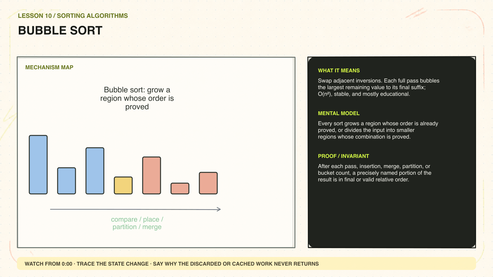
Watch from 0:00 ↗Swap adjacent inversions. Each full pass bubbles the largest remaining value to its final suffix; O(n²), stable, and mostly educational.
Bubble sort swaps adjacent inversions. After one full left-to-right pass, the largest value in the active prefix has crossed every smaller neighbor and reached its final position. Each later pass can ignore the finished suffix.
Walk through an example
[3,1,2] becomes [1,3,2] then [1,2,3]. The value 3 bubbles to the last position in the first pass; a pass with no swaps proves the array is sorted.
In an interview
Use it to explain invariants and stability, not as the default implementation. Worst-case time is O(n²).
Concept 2 of 6
Insertion sort
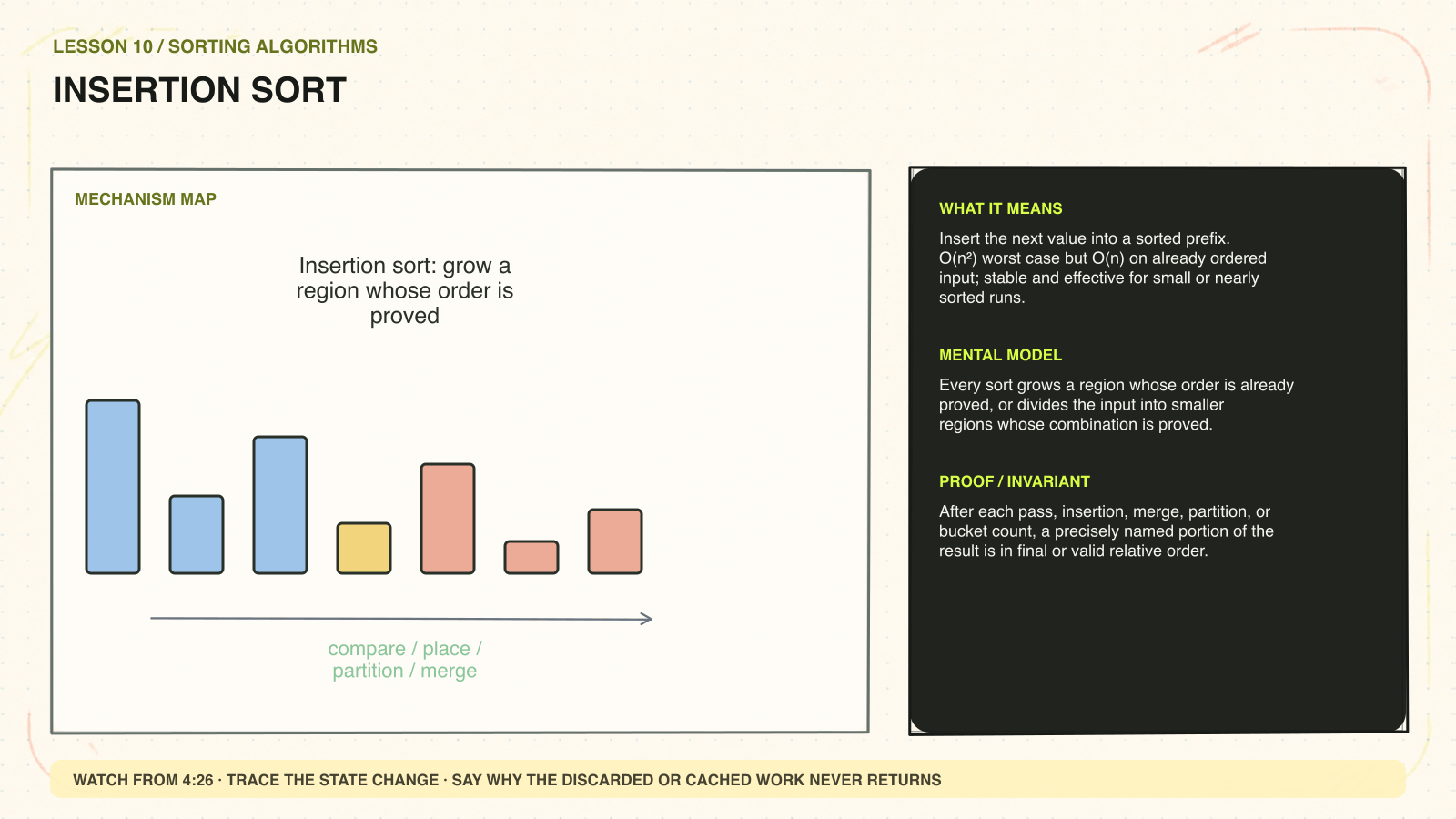
Watch from 4:26 ↗Insert the next value into a sorted prefix. O(n²) worst case but O(n) on already ordered input; stable and effective for small or nearly sorted runs.
Insertion sort maintains a sorted prefix. It takes the next value, shifts larger prefix values right, and inserts into the created gap. Work is proportional to the number of inversions, so nearly sorted input can be close to linear.
Walk through an example
With sorted prefix [1,4,7] and next value 3, shift 7 and 4 right, then place 3 after 1. The prefix [1,3,4,7] is sorted again.
In an interview
State that it is stable when equal items are not moved past one another, in-place, O(n²) worst case, and O(n) on already sorted input.
Concept 3 of 6
Selection sort
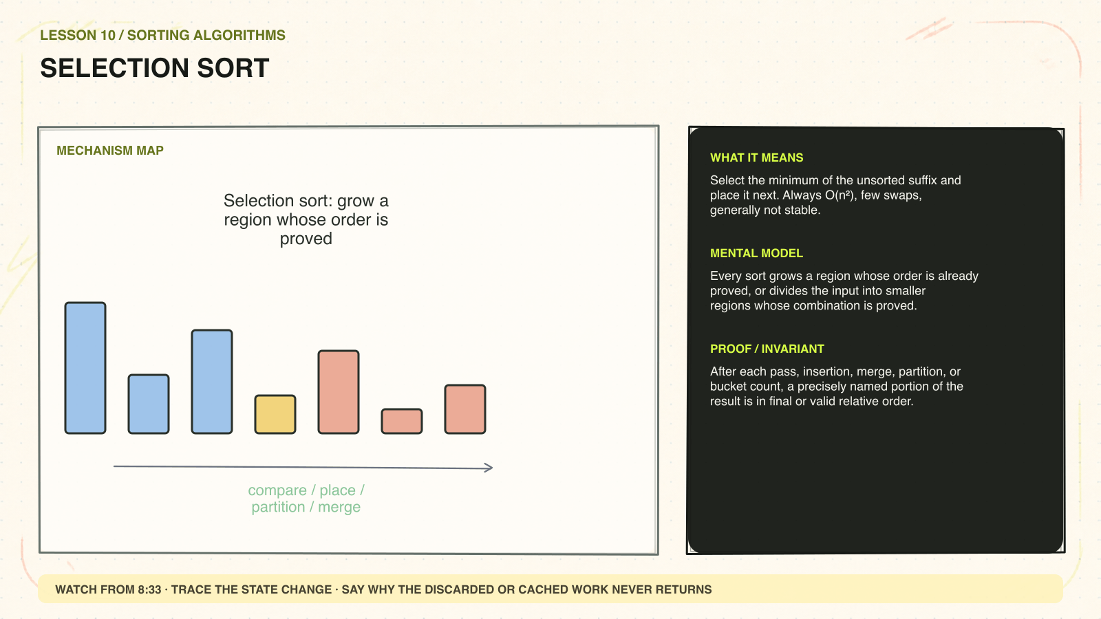
Watch from 8:33 ↗Select the minimum of the unsorted suffix and place it next. Always O(n²), few swaps, generally not stable.
Selection sort scans the unsorted suffix for its minimum and swaps that value into the next output position. The prefix grows by one correct final value per pass. It performs quadratic comparisons even when the input is already sorted, though it uses relatively few swaps.
Walk through an example
For [3,1,2], find 1 and swap it into index 0; then find 2 in the remaining suffix and place it at index 1.
In an interview
Contrast it with insertion sort: selection minimizes swaps but is generally unstable and receives no nearly-sorted speedup.
Concept 4 of 6
Merge sort
Watch from 11:54 ↗Recursively sort halves, then merge two sorted streams. O(n log n), stable, and typically O(n) auxiliary space for arrays.
Merge sort divides until subarrays are trivially sorted, then merges two sorted streams by repeatedly taking the smaller front value. Each level processes all n values, and there are log n levels, producing O(n log n) time.
Walk through an example
Merge [1,4] and [2,3]: take 1, then 2, then 3, then append remaining 4. Each pointer only advances, so the merge itself is linear.
In an interview
Mention stability, predictable O(n log n) time, and typical O(n) auxiliary array space. Linked-list merging can use different space behavior.
Concept 5 of 6
Quick sort
Watch from 23:30 ↗Partition around a pivot, then recurse. Average O(n log n), worst O(n²), commonly in-place, and highly sensitive to pivot and duplicate handling.
Quick sort partitions values relative to a pivot, then recursively sorts the partitions. Good pivots keep recursion balanced; consistently extreme pivots create quadratic work and linear depth. Partition details determine how duplicates and the pivot itself are handled.
Walk through an example
Around pivot 5, rearrange so values less than 5 occupy one region and greater values another. Once 5 reaches its final partition position, it never needs to move again.
In an interview
Give average O(n log n), worst O(n²), and explain pivot strategy or randomization rather than presenting the average as guaranteed.
Concept 6 of 6
Counting sort
Watch from 30:38 ↗Count each bounded integer key, then reconstruct order. O(n+k) time and O(k) space; it trades comparison generality for a finite key range.
Counting sort abandons comparisons when keys come from a manageable finite range. Count occurrences, convert counts to positions if stability is needed, and reconstruct the result. The range size k is part of both time and space.
Walk through an example
For [2,1,2,0], counts are [1,1,2]. Reading counts in key order emits [0,1,2,2] without comparing input values to one another.
In an interview
Check that k is not enormous relative to n and clarify how negative keys or associated records would be handled.
Before you call this lesson done
- Name the maintained sorted region
- State stability and auxiliary space
- Explain average versus worst case
- Use sorting when the resulting order enables a provable scan